

About me
srkobakian
Master of Philosophy in Statistics (QUT)
Bachelor of Commerce, Bachelor of Economics
I live in Melbourne, Australia

Ask me a question
Use the chat
Answer in discussion time
What can you do with ggplot2?
Use the Grammar of Graphics to build visulisations

What is the geom for mapping?
This is not a simple question
There are many types of maps
ggplot2: Elegant Graphics for Data Analysis:
Mapping Data
ggplot(Australia) + geom_point(aes(x = long, y = lat))
ggplot(Australia) + geom_line(aes(x = long, y = lat))
Polygon Mapping
ggplot(Australia) + geom_polygon(aes(x = long, y = lat, group = group))
This is a great start
- It looks like Australia!
- Borders are clear
- Islands are also clear
How can we improve this?
Simple Features
Key difference:
geometry list-column
Converts many, many rows
into a single row per area
Geometries fit together,
like puzzle pieces
ozmaps package
library(sf)library(ozmaps)sf_oz <- ozmap_data("country")sf_oz %>% kable()| NAME | geometry |
|---|---|
| Australia | MULTIPOLYGON (((144.8691 -4... |
ggplot(sf_oz) + geom_sf()
| NAME | geometry |
|---|---|
| New South Wales | MULTIPOLYGON (((150.7016 -3... |
| Victoria | MULTIPOLYGON (((146.6196 -3... |
| Queensland | MULTIPOLYGON (((148.8473 -2... |
| South Australia | MULTIPOLYGON (((137.3481 -3... |
| Western Australia | MULTIPOLYGON (((126.3868 -1... |
| Tasmania | MULTIPOLYGON (((147.8397 -4... |
| Northern Territory | MULTIPOLYGON (((136.3669 -1... |
| Australian Capital Territory | MULTIPOLYGON (((149.2317 -3... |
| Other Territories | MULTIPOLYGON (((167.9333 -2... |
sf_states <- ozmap_data("states")ggplot(sf_states) + geom_sf()
Data: COVID LIVE Australia
library(rvest)library(polite)covid_url <- "https://covidlive.com.au/report/cases"covid_data <- bow(covid_url) %>% scrape() %>% html_table() %>% purrr::pluck(2) %>% as_tibble()covid_data## # A tibble: 9 x 5## STATE CASES OSEAS VAR NET## <chr> <chr> <int> <lgl> <int>## 1 Victoria 20,479 NA NA 0## 2 NSW 5,150 1 NA 1## 3 Queensland 1,323 2 NA 2## 4 WA 912 1 NA 1## 5 SA 610 NA NA 0## 6 Tasmania 234 NA NA 0## 7 ACT 118 NA NA 0## 8 NT 104 NA NA 0## 9 Australia 28,930 4 NA 4
Complete map data
| NAME | geometry | CASES | OSEAS | NET |
|---|---|---|---|---|
| New South Wales | MULTIPOLYGON (((150.7016 -3... | 5150 | 1 | 1 |
| Victoria | MULTIPOLYGON (((146.6196 -3... | 20479 | NA | 0 |
| Queensland | MULTIPOLYGON (((148.8473 -2... | 1323 | 2 | 2 |
| South Australia | MULTIPOLYGON (((137.3481 -3... | 610 | NA | 0 |
| Western Australia | MULTIPOLYGON (((126.3868 -1... | 912 | 1 | 1 |
| Tasmania | MULTIPOLYGON (((147.8397 -4... | 234 | NA | 0 |
| Northern Territory | MULTIPOLYGON (((136.3669 -1... | 104 | NA | 0 |
| Australian Capital Territory | MULTIPOLYGON (((149.2317 -3... | 118 | NA | 0 |
Choropleth Map
ggplot(covid_states) + geom_sf(aes(fill = CASES))
library(ggforce)ggplot(covid_states) + geom_sf(aes(fill = CASES)) + facet_zoom(xy = NAME == "Australian Capital Territory", zoom.size = 0.6)
Off we go!

Covid in Sri Lanka
What is this unknown district?
Complete map data
| geometry | DISTRICT | Count |
|---|---|---|
| MULTIPOLYGON (((551311.8 58... | AMPARA | 1410 |
| MULTIPOLYGON (((501928.5 71... | ANURADHAPURA | 428 |
| MULTIPOLYGON (((522825 5682... | BADULLA | 1060 |
| MULTIPOLYGON (((609877 5593... | BATTICALOA | 426 |
| MULTIPOLYGON (((400911.5 49... | COLOMBO | 26925 |
| MULTIPOLYGON (((425038.8 40... | GALLE | 1852 |
| MULTIPOLYGON (((430775.7 53... | GAMPAHA | 15669 |
| MULTIPOLYGON (((592923.3 45... | HAMBANTOTA | 539 |
| MULTIPOLYGON (((362968.6 76... | JAFFNA | 229 |
| MULTIPOLYGON (((411888.2 43... | KALUTARA | 5674 |
| MULTIPOLYGON (((520143.4 55... | KANDY | 3573 |
| MULTIPOLYGON (((432117.3 52... | KEGALLE | 1315 |
| MULTIPOLYGON (((415223 7518... | KILINOCHCHI | 80 |
| MULTIPOLYGON (((425843.2 63... | KURUNEGALA | 2040 |
| MULTIPOLYGON (((405858.7 70... | MANNAR | 198 |
Choropleth Map
Off we go!
We can use projections
A projection converts the 3D globe, into to a 2D representation
Common Projections
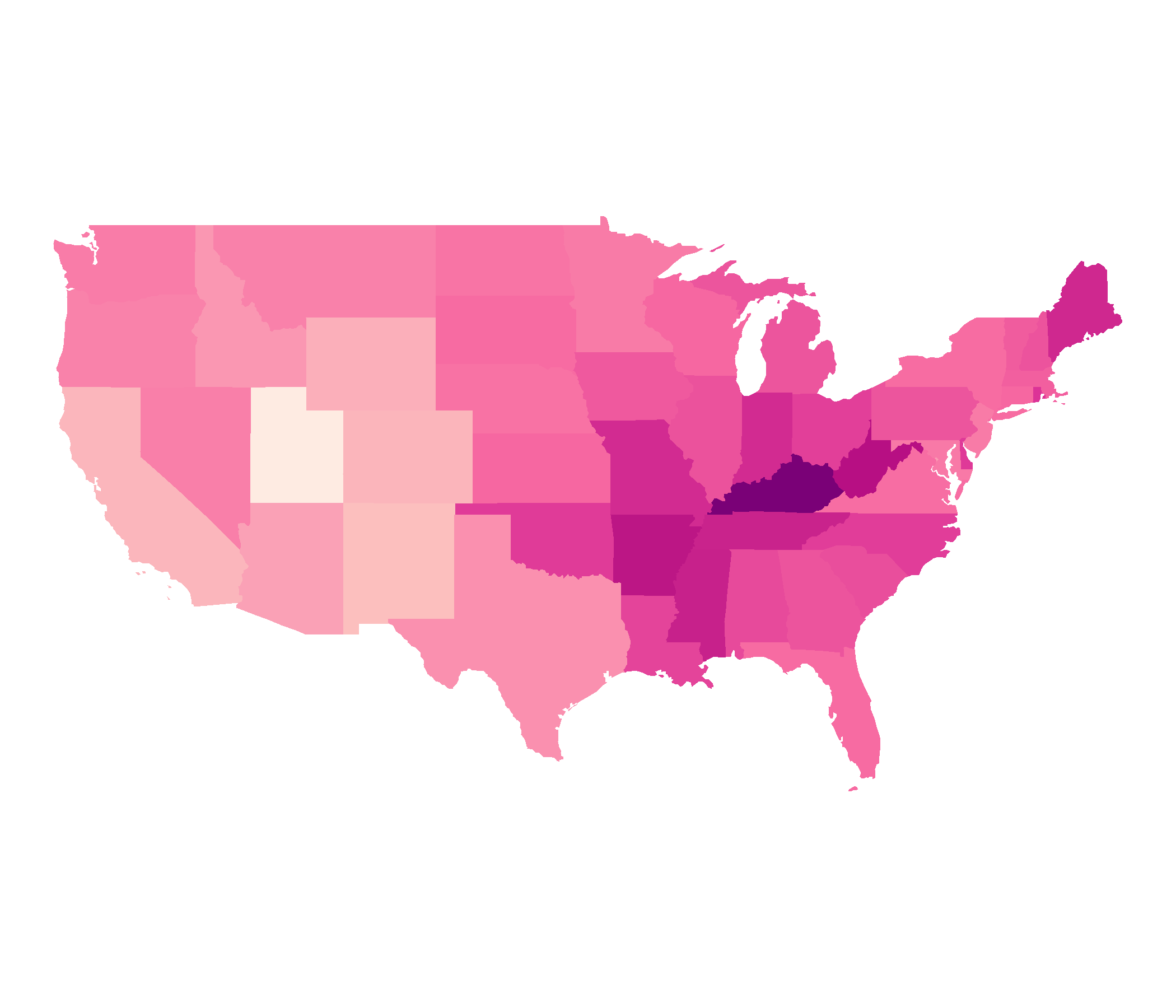
EPSG: 4326, World Geodetic System 1984, used in GPS
Common Projections
EPSG: 4326, World Geodetic System 1984, used in GPS
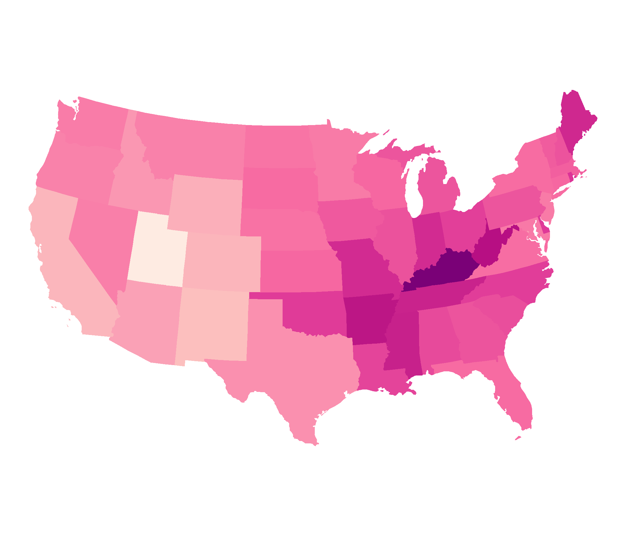
EPSG: 2163, US National Atlas Equal Area, spherical projection
Common Projections
EPSG: 4326, World Geodetic System 1984, used in GPS
EPSG: 2163, US National Atlas Equal Area, spherical projection
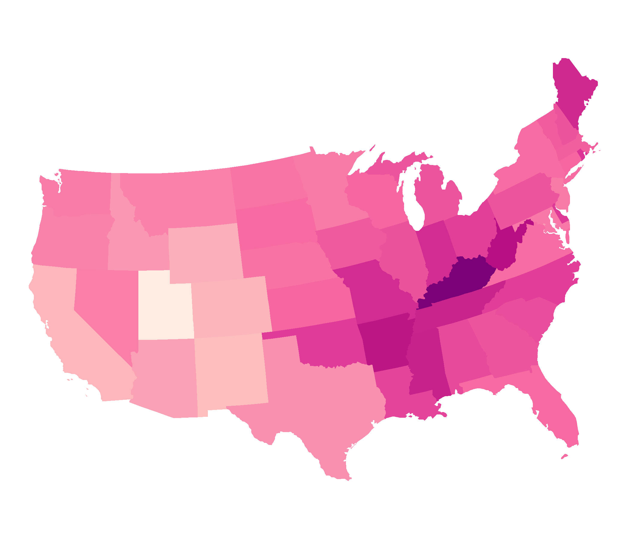
EPSG: 8826, North American Datum 1983
What are the alternatives?

Off we go!
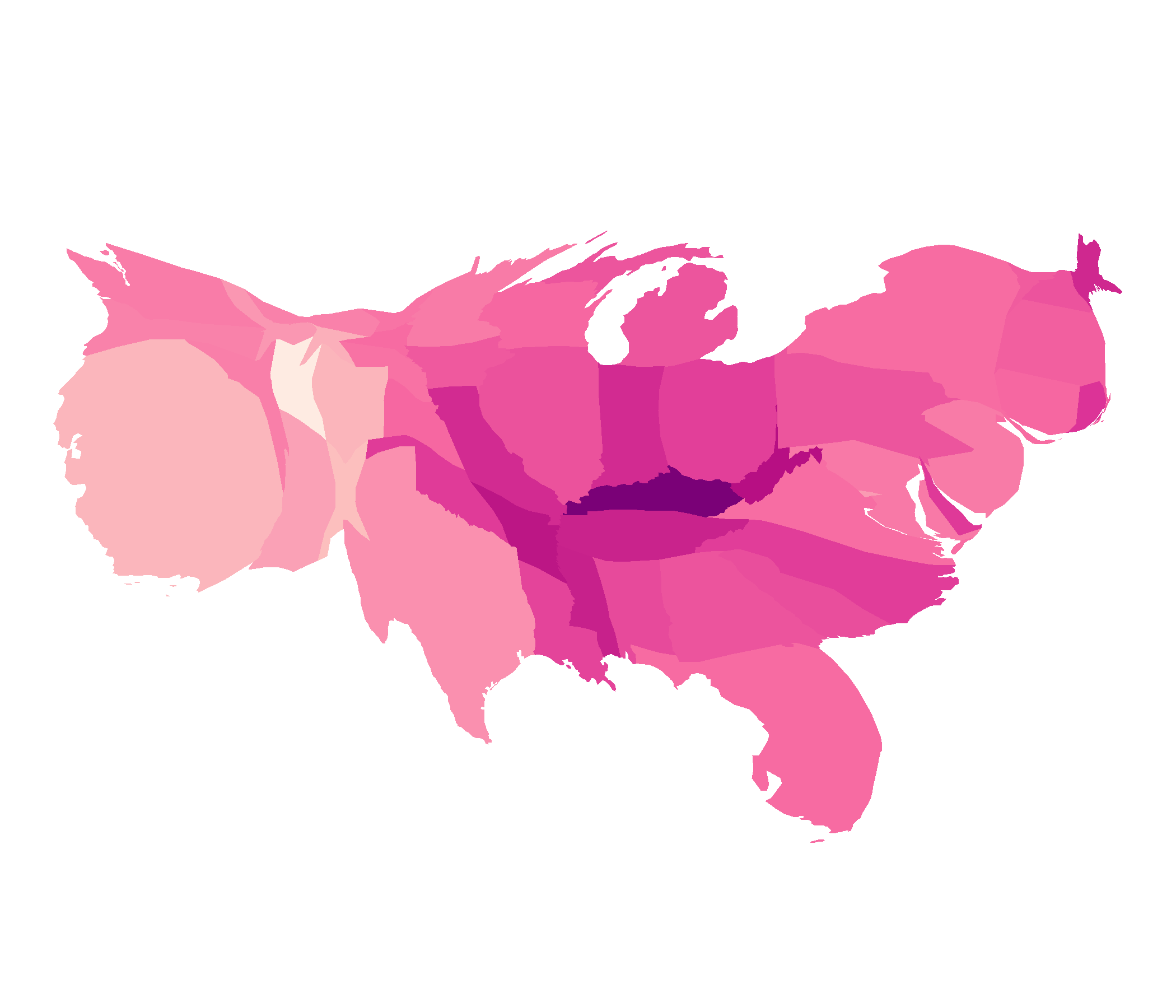
Contiguous Cartogram
library(cartogram)cont <- cartogram_cont(covid_districts_sl, weight = "population") %>% st_as_sf()ggplot(cont) + geom_sf(aes(fill = Count), colour = NA) + scale_fill_distiller(type = "seq", palette = "RdPu", direction = 1, ) + theme_map() + guides(legend.position = "right")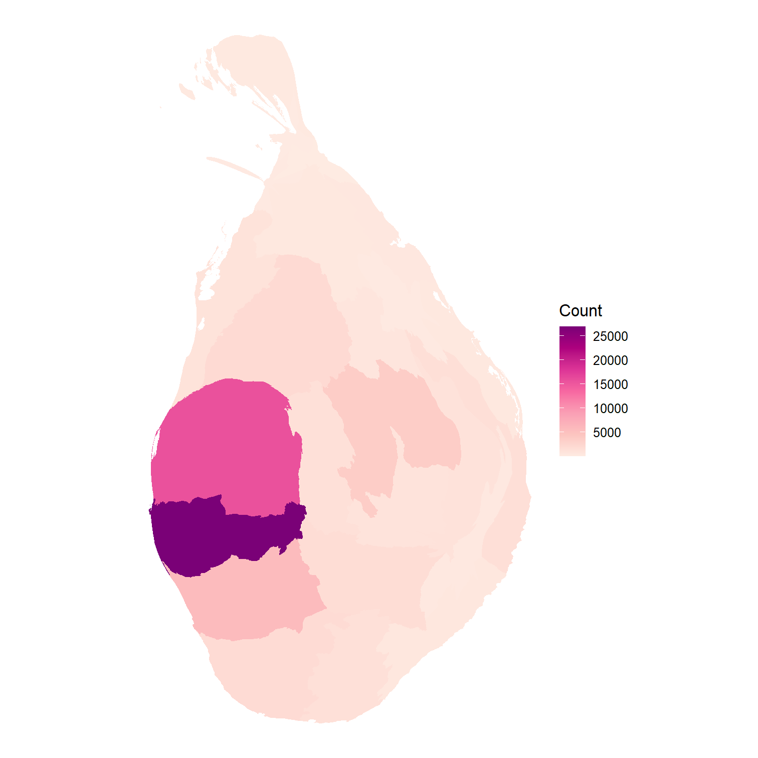
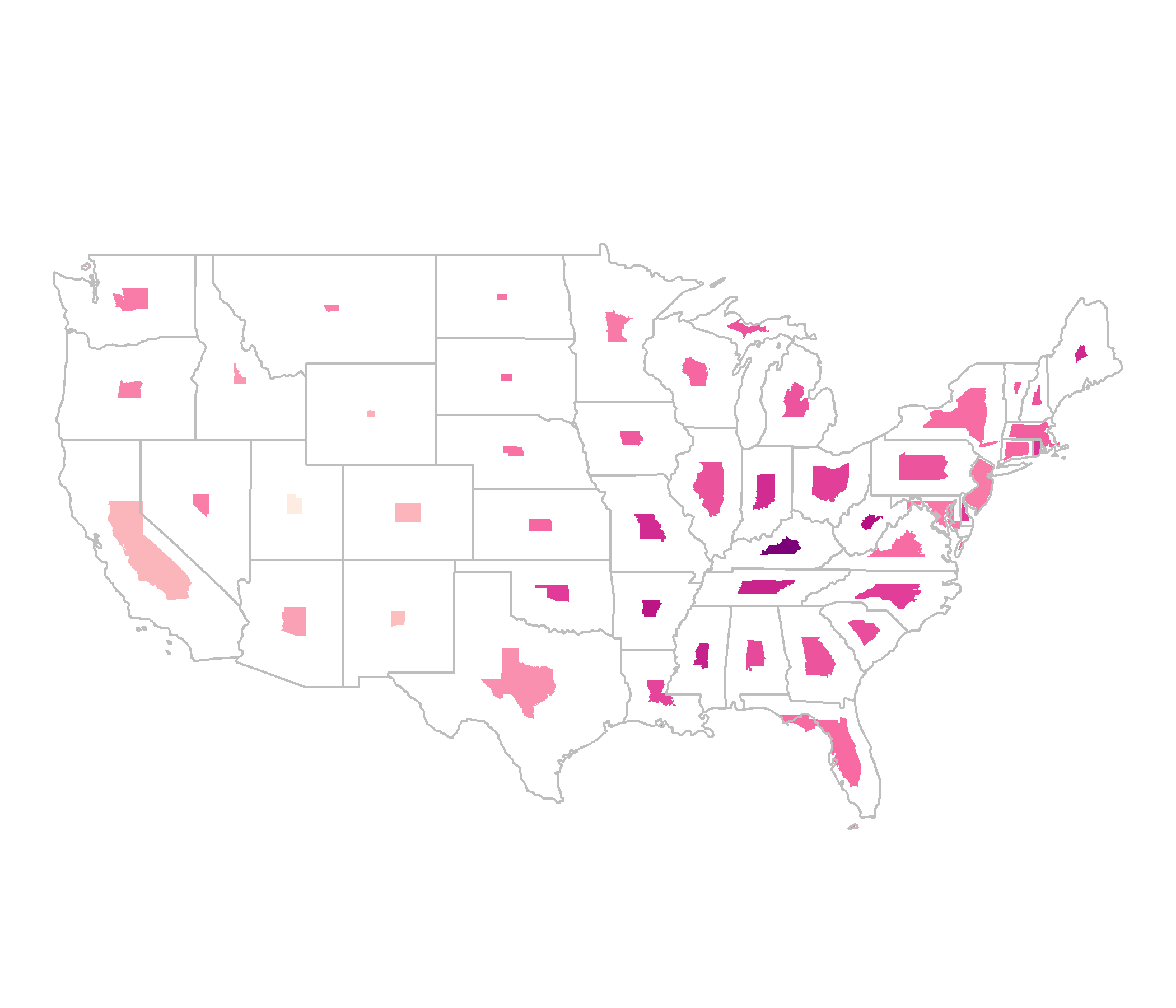
Non-Contiguous Cartogram
ncont <- cartogram_ncont(covid_districts_sl, weight = "population") %>% st_as_sf()ggplot(ncont) + geom_sf(data = covid_districts_sl) + geom_sf(aes(fill = Count), colour = NA) + scale_fill_distiller(type = "seq", palette = "RdPu", direction = 1) + theme_void() + guides(legend.position = "right")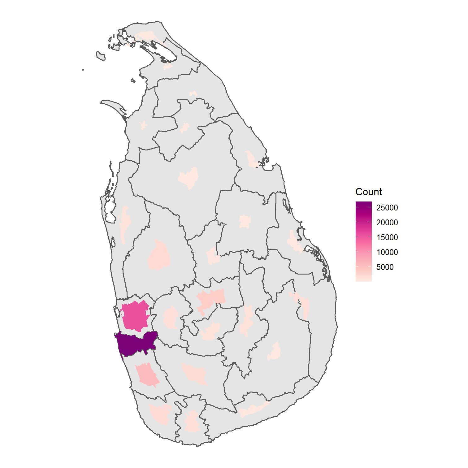
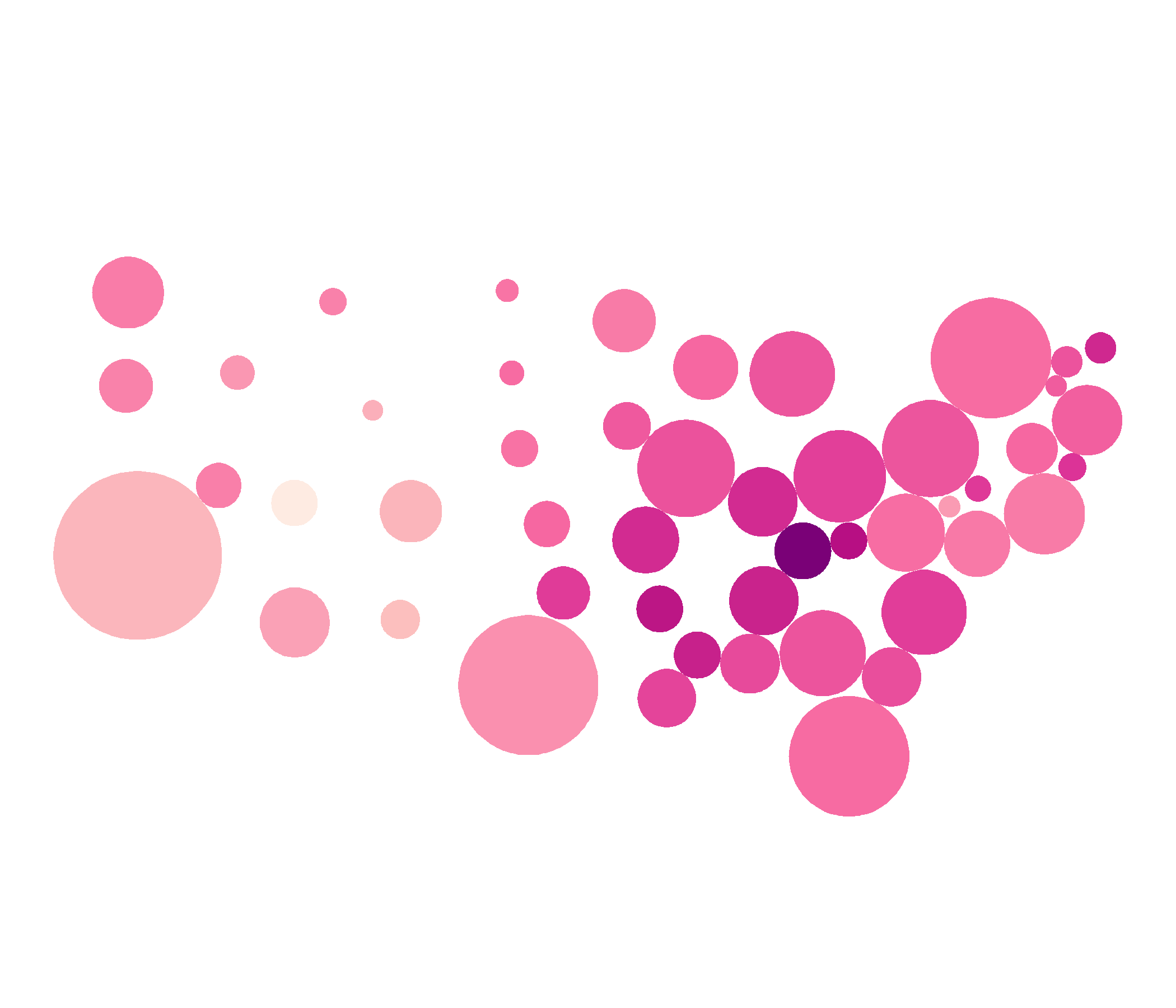
Dorling Cartogram
dorl <- cartogram_dorling(covid_districts_sl, weight = "population") %>% st_as_sf()ggplot(dorl) + geom_sf(data = covid_districts_sl) + geom_sf(aes(fill = Count), colour = NA) + scale_fill_distiller(type = "seq", palette = "RdPu", direction = 1) + theme_void() + guides(legend.position = "right")